Biodiversity Loss
Humans are causing the 6th mass extinction. How and why does that matter?
By Stephen Porder and Radika Bhaskar
Developed by the Laboratory for Educational Innovation at the Sheridan Center for Teaching and Learning
Between 1982 and 1984, the long-spined sea urchin (Diadema antillarum) population in the Caribbean declined precipitously—by almost 99%.
The urchins feed on algae. With the rapid decline in the urchin population, algae proliferated rapidly.
Hide text
As the algae overgrew the region, many corals were overrun with algae that was no longer eaten by sea urchins. In shallow waters around Jamaica, as much as 95% of coral reefs were covered by algae (Lessios 1988).
While there are many causes for coral reef decline in this region, the rapid loss of Diadema urchins was a major contributing factor.
Hide text
Staghorn Coral (Acropora cervicornus). Public Domain.
Today, there is at least some evidence that sea urchin populations can recover, aiding efforts to preserve corals in the Caribbean. But the case highlights the sometimes dramatic effects of biodiversity loss—that is, the loss of the variety of species in an ecosystem.
Hide text
Staghorn Coral (Acropora cervicornus). Public Domain.
This case is just one example of a much larger trend. According to the World Wildlife Fund, there has been a 52% decline in wildlife populations on Earth since 1970.
Hide text
Some species have become extinct, such as the golden toad (Bufo periglenes), which once lived in a small region of Costa Rica's northern cloud forests.
Hide text
Golden toad (Bufo periglenes). U. S. Fish and Wildlife Service. Public Domain.
Others, like the African elephant, are at extreme risk of extinction in the near future.
Hide text
There are many other charismatic examples, including polar bears, Florida panthers, and Siberian tigers.
Hide text
But the loss of charismatic, easy to see organisms, like polar bears, is only a small fraction of the loss of biodiversity that is happening today, and that will likely accelerate in the coming decades.
What this means for the organisms that go extinct is clear: extinction is forever. But the loss of biodiversity will have ramifications for the organisms that are still around.
Estimates vary widely, but there is little doubt that if habitat loss and climate change continue unabated, humans will be responsible for the sixth mass extinction event in the last 500 million years. What will this mean for the way our planet works? And for the species (like us) that are likely to survive?
One of the defining features of the Anthropocene is that the world is changing in ways that compel species to move, and another is that it's changing in ways that create barriers—roads, clear-cuts, cities—that prevent them from doing so.
Elizabeth Kolbert, The Sixth Extinction: An Unnatural History
In this module we'll explore three questions about human-driven losses in biodiversity:
-
What is biodiversity and how do we measure it?
-
What causes biodiversity loss?
-
What changes when biodiversity is lost?
What is biodiversity and how do we measure it?
Biodiversity encompasses the variety of life, at all levels of organization. Because this definition is so vast, trying to measure biodiversity can be tricky. For this module, we'll use the number of unique species as our estimate of biodiversity. But there are many other definitions: genetic diversity, diversity of whole ecosystems, etc.
If you walked into your backyard or a park in your hometown, how would you know how many unique speces are there? One way to answer that question would be to count them. This may be a relatively "easy" task for birds or mammals, but it is much more difficult to count insects or bacteria
For easily-identified groups, counting species seems simple enough in principle. In practice it presents many challenges.
Maybe the number of species is simply too large to count accurately. Maybe it's extremely difficult to find every species in a given area. Maybe you're not even sure what a species is.
So how do scientists go about measuring biodiversity? What can we do when we lack the means to count every species that exists on Earth?
One of the first studies that attempted to estimate the total number of species on Earth began by asking a much smaller, more focused question: how many different species of beetles live in the canopy of one tropical tree species, Luehea seemannii?
Hide text
Luhea seemannii. Rolando Perez and Richard Condit, Smithsonian Tropical Research Institute.
In the early 1980s, the entomologist Terry Erwin conducted a study in which he fumigated the canopy of nineteen individual trees, collecting everything that fell on a tarp below.
From this one tree species, Erwin identified neary 1000 different species of beetles.
Hide text
Luhea seemannii Flower, Fruit, and Leaf. Rolando Perez, Smithsonian Tropical Research Institute.
Based on his count, Erwin then began making educated guesses about global species numbers.
He used a variety of information from other studies:
-
Beetles account for roughly 40% of all known species.
-
On average, there are roughly 70 different tree species per hectare in the tropics.
-
Etc.
Erwin estimated that there may be as many as 30 million unique species on Earth—a much higher number than the working estimate at that time of only 1.5 million.
Was Erwin right? It turns out this is a question the scientific community is still attempting to answer.
Clearly, counting species by killing them, as Erwin did in the 1980s, is not an ideal solution for ecologists. So how are scientists going about estimating the total number of species on Earth? We largely rely on estimation, using information from sampling efforts.
One such effort has been ongoing for 30 years at Barro Colorado Island (BCI), in Panama.
Hide text
There, in one of the most-studied areas of tropical forest in the world, teams of scientists have been systematically surveying a 50 hectare plot (1000 by 500 meters) to develop a census of all woody trees and shrubs.
Every five years, each individual tree and shrub in the census plot is measured, mapped, and identified.
The resulting data can be used for many purposes, but we're going to use a subset of the BCI forest census data to illustrate some important principles—and critical challenges—involved in identifying the number of species in even a relatively small region.
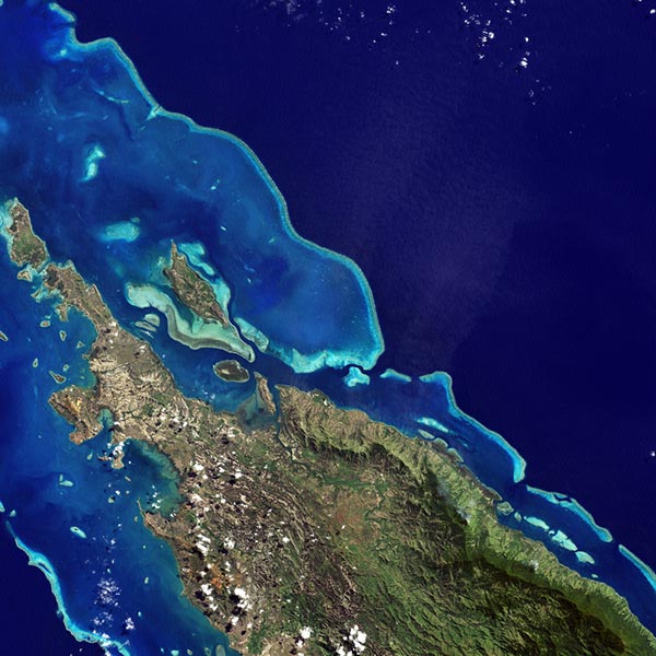
Hide text
Barro Colorado Island, Panama. NASA Earth Observatory
Imagine you want to identify the number of unique plant species found in a one hectare region of the main BCI plot.
You would begin by establishing a precise grid over the area you wish to survey. Let's start with a grid composed of squares that measure 20 meters on each side.
Next, you would conduct a survey of a single square—called a quadrat—to identify the species growing there.
Go ahead: click on any quadrat to select it to survey.
Using the actual data from the BCI forest, we see that the quadrat you've selected contains 0 total specimens—and 0 of those are unique species.
As we include more quadrats from the BCI dataset, you can see that surveying each quadrat in one hectare (100 x 100m) results in finding more and more species.
But there are diminishing returns. Each new quadrat has fewer new species and you find some you've seen in previous quadrats. Thus, the rate at which the number of new species are found slows down.
In this hectare, for instance, there are 0 total specimens, but only 0 unique species.
The rate at which new species are identified in the one hectare plot can be graphed to produce what is known as a species accumulation curve.
Rather than plot the number of trees, this curve plots the total unique species found against the number of quadrats surveyed.
A species accumulation curve is useful because it shows the relationship between sampling effort and unique species identified.
The steepest part of the curve occurs when surveying each new quadrat reveals many new species. As you continue surveying more quadrats, however, that rate begins to slow. In this case, 54% of unique species were found after surveying only eight quadrats.
This principle is involved in every sampling effort. When we want to measure diversity and the number of species is high (which is the case in many biological contexts) we must estimate based on the shape of this curve.
If we stop sampling too early, we risk underestimating dramatically. If we continue sampling, however, we find fewer new species with each additional unit of effort (which is time and money). Just for reference, surveying a 100m by 100m plot (1 hectare) might take about 2 weeks for a good team.
The abundance of a particular species also affects how likely we are to encounter it early in our sampling efforts. Most species are rare, so this is a real challenge.
This becomes even clearer if we examine a larger, ten hectare plot from the Barro Colorado Island data we've been using. You'll notice the plot is now elongated, 100 meters by 1000 meters, but each individual quadrat is still the same size.
Start surveying individual quadrats by clicking on them. As you do so, observe the species accumulation curve that is generated from your selections. How many unique species do you think you will find?
After surveying 0 quadrats, you've identified 0 total unique species. Try surveying another ten quadrats, then adjust your estimate based on what you observe.
You've now surveyed 0 quadrats and identified 0 total unique species. How accurate do you now think your estimate is? Try surveying another ten quadrats.
After 0 quadrats, you've found 0 total unique species. How many quadrats do you think you would need to survey to estimate accurately the total number of unique species in the full plot? Continue to the next slide to view the full species accumulation curve for this plot.
We see that roughly three quarters of the species in the plot are found in the first half of quadrats surveyed, with only 25% of species found in the remaining half.
How close was your final estimate to the total number of species actually identified in this BCI plot?
How valid is the estimate you can make from species accumulation curves like the ones we just seen? What are the limitations of this type of estimate?
If you were charged with surveying the biodiversity of this region, at what point on the curve would you feel you could make a statement about species richness in the area?
What does it matter if we don't count every species anyway? Why do we care about this aspect of biodiversity?
What causes biodiversity loss?
In 1963, Robert MacArthur and Edward Wilson published a new theory that tried to explain the number of species found on oceanic islands. The theory included the rate of immigration of species, the extinction rate, and the area of the island. The fact that the number of species in an place depends on the area of that place had been known for some time, particularly on islands. In fact, this observation underlies many subsequent attempts to estimate the loss of species caused by humans. But in the beginning, scientists interested in the species area curve (as the relationship is known) weren't motivated by understanding human impacts on the environment. Rather, they wanted to know what controlled the number of species found in a given area. Nonetheless, the observation that the number of species in a place seemed very strongly correlated with the area of that place. has been widely used to estimate human impacts on biodiversity.
Total number of reptilian and amphibian species on seven small and large islands in the West Indies. DennisM. Public Domain.
Original figure from MacArthur and Wilson The Theory of Island Biogeography 1967.
Many mechanisms have been proposed to explain the species-area relationship, and debate over those mechanisms is active today. But as people looked around the world, they found many other examples, such as plants in Australia and birds on different continents. See Rosenweig 1995 for a good book on this topic.
Hide text
A student of Wilson’s, Daniel Simberloff, decided to experimentally test whether area was really the control on the number of species. So he fumigated entire mangrove islands with methyl bromide, killing all the invertebrate animals. Then he returned each year to see how many species recolonized the islands.
He found the number of species that eventually recolonized the landscape was remarkably similar to the number that was there before. The relationship depended on how far the island was from the mainland (the source for recolonizing insects). Area alone did not explain the data. But area was a strong predictor of the number of species, before and after the fumigation/recolonization.
Fig. 2. The colonization curve of island E7. Source: Simberloff and Wilson Ecology 1969
If you’ve completed the submodule on quantifying biodiversity, the idea that the number of species you find is tied to the total area over which you search should be familiar. But it wasn’t long before people began to invert that thinking. Recognizing that humans were modifying the landscape (e.g. destroying habitat), people began to worry that a reduction in area would lead to a loss of species.
Imagine, for example, that half of Barro Colorado Island was cut down. How many species would you find in the remaining half of the island? How many species would you find if you cut down three-quarters of the island?
The idea that reduced area available for animals may lead to a reduction in the number of species is perhaps intuitive. However there is a big debate among ecologists and conservation biologists as to how big a risk area reductions pose.
Thomas et al. (2004) argued that climate change will reduce range sizes of organisms so much that 15-37% of species are threatened with extinction, and that these range size reductions may doom 10-15% of species to extinction in grasslands, boreal forests, and deserts. Not surprisingly, this paper got a lot of attention. 15-37% is a big number! And at the core of this argument is that smaller areas host fewer species (all other things held equal).
Other scientists quickly pointed out methodological flaws in Thomas et al's work. The debate continues to this day. In a paper with the refreshingly easy to understand (if provocative) title Species area relationships always overestimate extinction rates from habitat loss, He and Hubbell (2011) argue that the number of species lost as area is reduced is quite different from the number of species encountered when building a species accumulation curve. This too got a lot of attention, with several prominent scholars disagreeing with He and Hubbell.
The issue made the mainstream media.
For decades, it has been an open secret among conservationists. An elegant equation widely used to calculate how many species will go extinct from deforestation and habitat destruction -- one of the "laws" of ecological theory -- was a little shaky.
The New York Times, May 18, 2011.
The debate about how many species will go extinct because of habitat loss, how fast they will go extinct, and how things like connectivity between habitat fragments affects the number of species in an area, remains very active.
One thing is clear, however. While estimates vary widely, there is no doubt that habitat degradation and loss (e.g. reduced area) will be a key driver in determining the diversity of our planet moving forward.
And of course, habitat loss is not the only concern. Climate change may force species to migrate in order to survive. And often times, human modified landscapes stand in their way.
Hide text
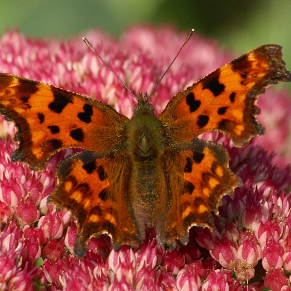
To illustrate how the combination of climate change and habitat loss might affect biodiversity, consider the very specific case of the silver-studded blue butterfly (Plebejus argus). Like any one species that isn’t a polar bear or similar charismatic animal, its loss may not cause much alarm. But the plight it faces is going to be faced by ever increasing numbers of species (plants and animals) in the coming decades.
Hide text
The range of the silver-studded blue extends across much of Europe and northern Asia as far west as Japan. While it remains common across much of its range, silver-studded blue populations in the United Kingdom have declined since the 1970s.
This animation shows the butterfly's decline in range from the 1970s to the late 1990s. While the differences may seem minor to the eye, by 1999 the silver-studded blue occupied 28% less land in the United Kingdom than it did just twenty years before.
Source: Warren et al. Nature 2001
During the same period as this decline in range, temperatures in the United Kingdom have been warming. As a result, temperatures across a larger portion of the UK are now suitable for the silver-studded blue.
These regions, shaded dark blue on the map above, are areas where the butterfly could live—yet, for some reason, it does not. Why might this be the case?
Source: Warren et al. Nature 2001
The answer to this question involves studying the interrelation of suitable habitat and suitable climate for a given species.
To illustrate how habitat and climate interact, let's start with a very simple abstract representation. This graphic illustrates the simplest possible scenario, in which a species—in this case, the silver studded blue—exists in some unspecified area of land. Here, the shaded box indicates this land area.
Not all land provides a suitable habitat for a species, however. For example, the silver-studded blue favors lowland heaths and grasslands, where the heathers, vetches, and other plants that supply the larvae and butterflies with sources of food are commonly found.
As a result, the butterfly can live only in those areas that contain suitable habitat.
The suitability of climate also determines what areas a species can occupy, even when suitable habitat is available. The silver-studded blue is an example of a thermally limited species, meaning that it can only live within a specific range of temperatures. In areas where the temperatures are lower than what it requires, the butterfly cannot survive.
Consequently, as this graphic illustrates, the silver-studded blue's range is limited to areas where suitable habitat and suitable climate coincide.
The areas where suitable climate and suitable habitat coincide determine the butterfly's range. Within these areas the butterfly can disperse freely, represented here by arrows.
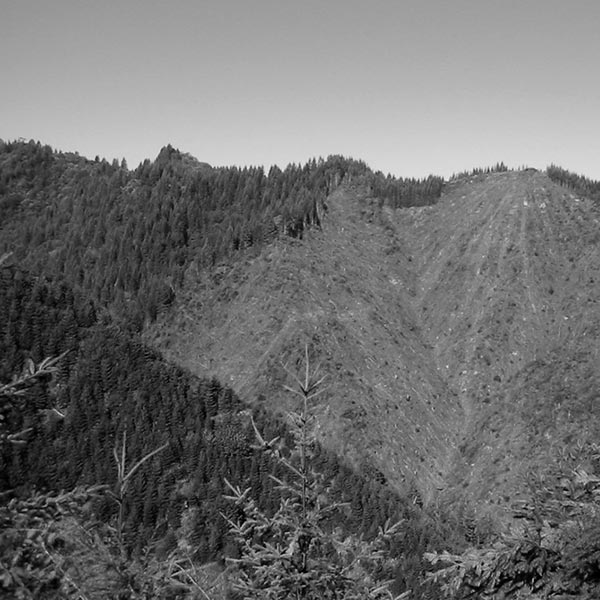
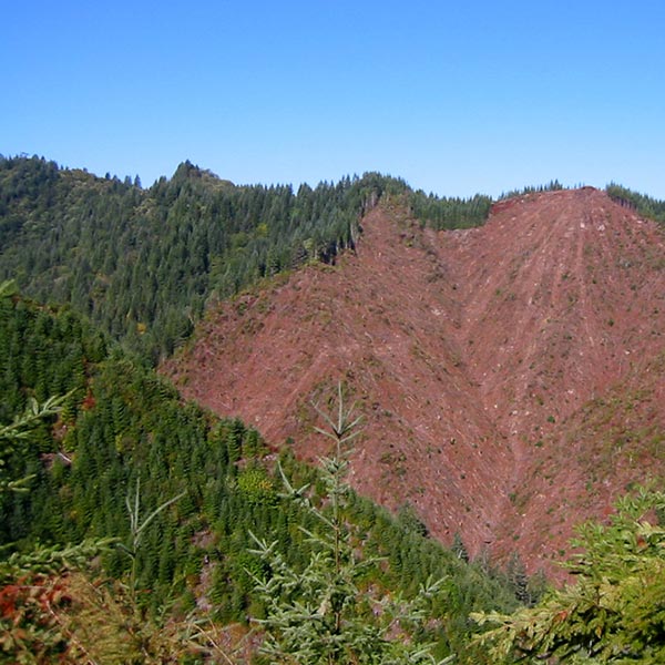
But there is another factor that complicates matters for the silver-studded blue: habitat loss caused by various human activities.
As habitat loss occurs, whether through agriculture or urbanization, areas where climate and habitat are both suitable for the butterfly become smaller and more fragmented.
Initially, populations of the butterfly may be able to move between some of the remaining habitat fragments, particularly those that are not separated by large distances.
However, a species like the silver-studded blue has low mobility and relatively specialized habitat requirements, so even small amounts of habitat loss or fragmentation pose a threat. Its inability to survive in farmland or urban gardens means that its range will be restricted to the remaining patches of natural vegetation.
With warming temperatures, regions to the north that were previously too cold for the silver-studded blue to survive become habitable. But because of its low mobility and the fragmentation of its natural habitat, the butterfly is unable to disperse to these areas.
Instead, it remains limited to the remaining habit that it can still reach within its previous range.
If warming continues, southern regions that the butterfly once occupied may become too hot for it to survive, even if some habitat remains. The northward movement of the suitable climate window for the silver-studded blue will further diminish the areas where it can thrive.
This combination of changing climate and habitat loss places the silver-studded blue at risk for local extinction within the United Kingdom. If climate change or further human activities cause the patches the butterfly now occupies to disappear, it will not be able to disperse to the areas made newly habitable by warming temperatures further north.
This explains the map we saw earlier, comparing the silver-studded blue's current range (regions shaded light blue) and the range it could occupy if it were more mobile and less affected by habitat fragmentation. This map suggests that although suitable habitat and climate may exist elsewhere in the United Kingdom, the butterfly is simply unable to reach these areas.
Source: Warren et al. Nature 2001
Further complicating our understanding of the drivers of biodiversity loss is the delay between environmental perturbations and the eventual disappearance of a species. During this lag, or period of decline, individuals of a species remain present, so the threat to the species as a whole can often be overlooked.
This is sometimes referred to as extinction debt, a term that describes the number of species expected to become extinct eventually due to some past disturbance.
What are the consequences of biodiversity loss?
How can we test if losing biodiversity matters? We have reasons to suspect it does, but we must ask “matters for whom?” and “how do we quantify how much it matters?”
Obviously, species that are lost are affected by biodiversity loss. But what about those that remain? Those species, humans included, depend on ecosystems for the provision of food, water, and fiber. How can we tell if those provisions will be affected by a loss of biodiversity?
Scientists have taken several approaches to address this question, two of which we’ll focus on here: experimental manipulations and observational studies.
Hide text
Perhaps the best-known test of the importance of biodiversity for ecosystem function comes from a long-running experiment in Cedar Creek, Minnesota. As you can see in this airphoto, the landscape looks like a series of neat squares.
Hide text
Courtesy: LTER Network Office
What you can’t see from the air is that each square is planted with the same number of individual plants, but with different numbers of species. Plots contain 1, 2, 4, 8, 12 or 24 species.
Researchers have been monitoring how these different “ecosystems” function for the past 20 years, and have noted strong relationships between a variety of ecosystem functions and the number of species in the plots.
Hide text
Courtesy: LTER Network Office
Left: More species meant more productivity and plant cover. That means more habitat, but it also means more plants for us to use. Productivity is an important ecosystem function.
Right: The plots with more species were more resilient in the face of drought.
Redrawn from Tilman et al. Nature 1996 and Tilman and Downing Nature 1994
Left: The plots with more species were able to utilize more of the available nutrients.
Right: Fewer nutrients leach out. Since leached nutrients pollute waterways, the retention of nutrients is an important ecosystem function.
Redrawn from Tilman et al. Nature 1996
What can this experiment tell us?
Higher diversity leads to higher productivity, more efficient use of nutrients, and greater stability.
Hide text
But, at the end of the day, experimental plots, even those maintained for decades, are different from natural systems. What does this experiment tell us about the role of biodiversity in tropical forests, where there would be several hundred tree species in an area as big as the Cedar Creek experiment?
As is always the case, one experiment, or one type of experiment, does not give the whole story. While Cedar Creek has provided some of the strongest evidence to date for the importance of biodiversity in maintaining stable, productive ecosystems, it is only one line of evidence among many.
Hide text
A much more complicated, and controversial, observational study centers around the prevalence of Lyme disease, a bacterial infection first diagnosed in humans in 1975. While this story is less “experimental” it too offers insights into the dangers of biodiversity loss.
Since 1995, the United States has seen a steady increase in reported cases of Lyme disease.
Lyme disease is caused by the bacterium Borrelia burgdorferi. Humans contract the disease after being bitten by deer ticks (Ixodes scapularis) carrying this bacterium. The ticks themselves are not susceptible, meaning they are merely a vehicle for transmitting the disease to humans—so we consider them carriers or vectors.
Hide text
These ticks are commonly known as deer ticks because deer are frequent hosts and are able to host the ticks in large numbers.
For the past thirty years, there has been a widespread belief that large deer populations contribute to increased risk of infection in areas with high rates of Lyme disease. As a result, many states have implemented policies intended to reduce deer abundance, such as controlled deer hunts.
Hide text
Male white-tailed deer. U. S. Fish and Wildlife Service. Public Domain.
The evidence that deer are responsible for increasing human infection is not overwhelming, and in some cases there is no clear connection at all between deer density and disease rates.
This raises a critical question: if deer are not responsible for the spread of Lyme disease, what is?
Hide text
In order to answer that question, we need to understand the full life cycle of ticks and its relation to Lyme disease.
Ticks have three life stages. At each stage, the ticks require a blood meal before molting and moving to the next stage. Ticks hatch from eggs uninfected, meaning that each generation of ticks must acquire the Lyme bacterium in order to pass it on to a host.
The stage that poses the greatest risk to humans is the nymphal stage of development. The time of this stage coincides with the warmer months during spring and summer, when outdoor human activity tends to be highest. Ticks are also very small during this phase, making them more difficult for humans to see than during their adult phase.
Hide text
If the nymphs are responsible for transmitting the disease to humans, then they must have acquired the bacterium that causes Lyme disease earlier in their life cycle—during the larval phase. Tick larvae can feed on a number of different small mammals and birds, so some or all of these larval hosts must be involved in the ticks' initial acquisition of the Lyme-causing bacterium.
Hide text
It turns out these host organisms differ in important ways that influence Lyme disease transmission. They vary in body size, which influences the number of ticks that can feed on any given individual. They vary in how well they transmit the bacteria (depending in part on the host immune system). They also vary in how tolerant they are of hosting ticks, meaning some species groom themselves to pick off and/or eat ticks more than others.
These differences in attributes and behavior mean that when a wide array of hosts is present, it serves to moderate the transmission of Lyme infection. This effect has been termed the dilution effect.
Hide text
To illustrate basic concept of the dilution effect, we'll follow a population of 100 ticks through two scenarios that demonstrate how reductions in species diversity result in a higher percentage of ticks carrying Lyme disease.
In an unperturbed ecosystem, there are many species on which ticks may feed. Common mammals that host ticks include mice, deer, squirrels, and opossums. In many ecosystems, there are also other possible hosts, but we'll simplify for the purposes of illustration.
Imagine that 25 ticks feed on each of our four hosts. Again, this is a simplification, because in the wild more ticks will feed on some hosts than on others, and some potential hosts are more abundant than others.
After feeding, some of the surviving ticks from each host will be carrying Lyme disease. The percentage of ticks carrying the bacterium depends on how easily the it is transmitted from the host to the tick, and varies significantly by species. Around 90% of ticks that survive feeding on the white-footed mouse will carry it, while fewer than 10% of ticks feeding on deer will.
Of the original 100 ticks, roughly 50% survive and leave their hosts. (The other ticks are groomed off their hosts or die for other reasons.)
In this unperturbed ecosystem with high diversity, roughly twelve of the fifty surviving ticks will be carrying Lyme disease. That's just below 25% of the remaining tick population, and these ticks will now be able to transmit Lyme disease to a future host—perhaps to a human.
What would happen if species diversity were reduced in this ecosystem, leaving ticks with fewer species on which to feed?
To answer that question, let's consider the case of a perturbed ecosystem in which white-footed mice are extremely abundant.
Now, instead of feeding on several different species, the original 100 ticks feed exlusively on mice.
In the previous example, ticks that survived feeding varied in the rate at which they carried the bacterium causing Lyme disease, depending on the host. Now, however, because white-footed mice transmit the Lyme bacterium to ticks very efficiently, ticks feeding on every host have a high likelihood of carrying the bacterium.
This means that a much higher percentage of the surviving tick population—46 out of 50 surviving ticks, or 92%, in this simplified example—now carry the bacterium in the perturbed ecosystem scenario. With so many ticks carrying the bacterium causing the disease, the likelihood of transmission to humans increases dramatically.
We can see the outcome of the dilution effect for human Lyme risk when we look at different states, with different levels of species richness of small mammals.
This graph shows the strong relationship between species richness and rate of Lyme disease cases in humans; states with greater small mammal species richness generally have much lower rates of human infection.
How does this explain the original pattern of increasing Lyme incidence? To understand that we have to look at how we have changed the habitat, in this case the forest landscape. Much of the formerly continuously forested land has been cleared leaving small patches or fragments of forest behind. Forest fragmentation leads to a higher incidence of infected ticks. Why?
As is covered in the submodule about causes of biodiversity loss, when the area of forest is decreased the number of species that can be supported is reduced. And while most species are not common in small patches, it turns out white-footed mice are abundant in small areas.
Increasingly humans live in suburban landscapes, near very small patches of forest, putting them in close proximity with high mice density, and therefore high infected nymph density. This is one of the big factors that seems to contribute to Lyme incidence.
Hide text
Lyme may be but one example illustrating the impact of biodiversity on infectious disease. Other similar observations have been made in different systems. For example, amphibians have a reduced risk of contacting a pathogen that leads to leg deformities when they live in more species rich communities.
The role of biodiversity in moderating infectious lyme disease risk is not universally accepted. There are many diverse, relatively intact ecosystems (think tropical forests) where disease risk is high. There are are super low diversity ecosystems (think New York City) where your risk of lyme disease is relatively low. Much more science will need to be done to flesh out the role of biodiversity in providing the things humans need from ecosystems.
Conclusion
Can anything be done about biodiversity loss?
The loss of biodiversity is likely to proceed rapidly in the coming decades, as climate change exacerbates the effects of habitat loss and fragmentation. The data from the Cedar Creek experiment demonstrates some of the value of biodiversity, and fit pretty well with what we would predict from ecosystem theory. But the Lyme disease example highlights how losses of biodiversity can have completely unexpected results that are difficult to untangle.
Conservation biologists, land managers and policy makers have to deal with two simultaneous threats. Climate change will force species to migrate. And habitat loss threatens to both destroy where species live and prevent their climate-driven migration. Are there answers to this two pronged threat?
In marine systems, biologists are trying to understand how marine reserves where fishing is limited can serve to increase fish populations, support healthy populations of fish and fishermen, and help buffer populations against the impacts of climate change.
On land it has long been recognized that protected areas are not enough. There is simply not enough land to set aside to conserve high levels of biodiversity. People are working to restore habitat, protect what is left, and connect places currently separated by human-dominated landscapes. Organizations like the The Nature Conservancy, World Wildlife Fund and many others work all over the world in partnership with local governments and stakeholders.
There is still much work to be done. Here at Brown, Professor Dov Sax's lab (http://www.brown.edu/Research/Sax_Research_Lab/) tries to understand how species will adapt, migrate, or go extinct as a result of climate change.
At the Hopkins Marine Station in Monterrey Bay, CA Stanford Professor Steve Palumbi (http://palumbi.stanford.edu/) is trying to understand how corals may evolve resistance to warming seas.
The Natural Capital Project (http://www.naturalcapitalproject.org/) seeks to quantify the values that ecosystems provide to people in the hopes that this will spur conservation and innovation.
Hide text
There are many other examples. Conservation, like agricultural sustainability and stopping climate change, will require both excellent science and sound policy. Think about if, and where, you want to gain expertise so you can make your contribution.
References
Kolbert E (2014). The Sixth Extinction: An Unnatural History.
Lessios HA (1988). Mass mortality of Diadema antillarum in the Caribbean: what have we learned? Annual Review of Ecological Systems 19:371–393.
Lovett RA (2006). Endangered Species List Expands to 16,000. National Geographic News.
Rankin B (2009). World Cropland. Radical Cartography.
World Wildlife Fund (2014). Living Planet Report 2014: Species and spaces, people and places.
About
This module was written by Stephen Porder and Radika Baskhar, and developed by the Laboratory for Educational Innovation at Brown University's Sheridan Center for Teaching and Learning.